Entry #12 Image Processing and ML on my Snack
- jamescgonzales
- Feb 1, 2021
- 6 min read
Applications of Image Processing in Machine Learning Python.

With all the previous posts published, I decided to take a break. I indulged myself with a little junk food. While savoring the unhealthy food that will make me more obese than I am now, I noticed the size and shape of the things I have been putting into my mouth. Can I do Image Processing and apply Machine Learning on my Snack? Let's try. :)
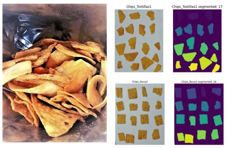
Pic-A is a combination snack brand from the same maker- Jack ‘n Jill. It is composed of other brands of chips from Nova, Piattos, Tostillas, and air. (I am kidding on the last..., or do I?)
I sorted out the chips based on their brand and took a photo, and saved them with their filename based on their brand. The filename's format is "Chip_{Brand}#.jpg"
The images will be segmented to extract their features.
Once the data is extracted, it will be stored in pandas data frame for train-test splitting and input to various Classification Machine Learning algorithms.
So now, let's begin.
Like before, let's import the python libraries needed.
import os
from glob import glob

import re
import time
import numpy as np
import pandas as pd
import matplotlib.pyplot as plt
import matplotlib.gridspec as gridspec
from scipy.signal import convolve2d
from skimage.io import imread, imshow
from skimage.color import rgb2gray
from skimage.measure import label, regionprops, regionprops_table
from skimage.transform import rotate
from skimage.morphology import (erosion, dilation, closing, opening,
                                area_closing, area_opening)
from sklearn.preprocessing import MinMaxScaler, StandardScaler
from sklearn.model_selection import train_test_split
from sklearn.neighbors import KNeighborsClassifier
from sklearn.linear_model import LogisticRegression
from sklearn.svm import LinearSVC
from sklearn.svm import SVC
from sklearn.naive_bayes import GaussianNB
from sklearn.tree import DecisionTreeClassifier
from sklearn.ensemble import GradientBoostingClassifier
from sklearn.ensemble import RandomForestClassifier
I also pre-prepared the morphological functions and structuring element
sel_h = np.array([[0, 0, 0],
                  [1, 1, 1],
                  [0, 0, 0]])

sel_v = np.array([[0, 1, 0],
                  [0, 1, 0],
                  [0, 1, 0]])

sel_c = np.array([[0, 1, 0],
                  [1, 1, 1],
                  [0, 1, 0]])

blur = (1 / 16.0) * np.array([[1., 2., 1.],
                              [2., 4., 2.],
                              [1., 2., 1.]])

def multi_dil(im, num, sel=None):
    for i in range(num):
        im = dilation(im, sel)
    return im


def multi_ero(im, num, sel=None):
    for i in range(num):
        im = erosion(im, sel)
    return im
Here's the properties or features that will be extracted from the chips.
properties = ['area', 'centroid', 'convex_area', bbox', 'bbox_area
              'eccentricity', 'equivalent_diameter',
              'extent', 'filled_area', 'major_axis_length',
              'minor_axis_length', 'mean_intensity',
              'perimeter', 'orientation', 'solidity']
Image Segmentation
Now given the image files, let's segment the chip images for every group. Let's start with the "Nova Chips"
Segmenting Nova Chips
We can validate if we are getting the right files, by getting the length of the file variable from glob
Here's the code for the segmentation. It already includes the thresholding and morphological adjustment of the image in order to extract the correct number of objects of interest.
clean_chips_nova = []  # List of two tuples (img, regionprops)
fig = plt.figure(figsize=(20, 20))
file_count = len(chips_nova_files)
thres = 0.633
no_col = 4

no_row = int(np.ceil(file_count * 2 / no_col))

gs = gridspec.GridSpec(no_row, no_col)

for i, file in enumerate(chips_nova_files):

    img = imread(file)
    fn = file.split('\\')[-1].split('.')[0]
    ax0 = fig.add_subplot(gs[i * 2])
    ax1 = fig.add_subplot(gs[i * 2 + 1])
    ax0.axis('off')
    ax1.axis('off')


    # Display Threshold Image
    ax0.imshow(img)
    ax0.set_title(fn)

    # Threshold image
    img = rgb2gray(img)
    img_bw = img < thres

    # Morph Image
    img_morph = area_closing(area_opening(img_bw, 200), 200)
    img_morph = multi_ero(multi_ero(img_morph, 22, sel_v), 2, sel_h)
    img_morph = multi_dil(img_morph, 20, sel_v)

    # Get region properties of image
    img_label = label(img_morph)
    df_regions = pd.DataFrame(regionprops_table(img_label, img,
                                                properties=properties))

    # Filter regions using area
    area_thres = df_regions.convex_area.mean()/3
    df_regions = df_regions.loc[df_regions.convex_area > area_thres]

    mask_equal_height = ((df_regions['bbox-2'] - df_regions['bbox-0'])
                         != img_label.shape[0])
    mask_equal_width = ((df_regions['bbox-3'] - df_regions['bbox-1'])
                         != img_label.shape[1])
    df_regions = df_regions.loc[mask_equal_height & mask_equal_width]

    # Compute for Derive features
    y0, x0 = df_regions['centroid-0'], df_regions['centroid-1']
    orientation = df_regions.orientation
    x1 = (x0 + np.cos(df_regions.orientation) * 0.5
          * df_regions.minor_axis_length)
    y1 = (y0 - np.sin(df_regions.orientation) * 0.5
          * df_regions.minor_axis_length)
    x2 = (x0 - np.sin(df_regions.orientation) * 0.5
          * df_regions.major_axis_length)
    y2 = (y0 - np.cos(df_regions.orientation) * 0.5
          * df_regions.major_axis_length)

    df_regions['major_length'] = np.sqrt((x2 - x0)**2 + (y2 - y0)**2)
    df_regions['minor_length'] = np.sqrt((x1 - x0)**2 + (y1 - y0)**2)
    df_regions['circularity'] = (4 * np.pi * df_regions.filled_area
                                 / (df_regions.perimeter ** 2))

    # Display segmented image
    ax1.imshow(img_label)
    ax1.set_title(f'{fn} segmented: {df_regions.shape[0]}')

    df_regions['target']='chips_Nova'
    clean_chips_nova.append(df_regions)
Based on the number of segment and the actual chips, the image was correctly segmented.
2. Segmenting Piattos Chips
For Piattos chips, instead of using grayscale threshold, I used the hsv filtering method below.
    image_hsv = rgb2hsv(img)
    lower_mask = image_hsv[:,:,0] > 0.08
    upper_mask = image_hsv[:,:,0] < 0.4
    sat_mask = image_hsv[:,:,1] < 1
    img_bw = upper_mask*lower_mask*sat_mask
3. Segmenting Tostillas Chips
We Tostillas. I used 0.6 threshold grayscale filter.
    img = rgb2gray(img)
    img_bw = img < 0.6
Based on the samples collected, it is obvious that the most of the brand inside my Pic-A are Novas.
Next is to combine the dataframe
df_chips = pd.concat([*clean_chips_nova, *clean_chips_piattos,
                      *clean_chips_tostillas])
Then we will just retain the we will be using on our machine learning.
req_feat = ['area', 'convex_area', 'bbox_area', 'eccentricity',
            'equivalent_diameter', 'extent', 'filled_area',
            'perimeter', 'mean_intensity',
            'solidity', 'major_length', 'minor_length',
            'circularity', 'target']
df_chips = df_chips[req_feat]
Setting up our Machine Learning models
Here are the features and the target
X = df_chips.drop('target', axis=1)
y = df_chips.target
We will split the dataset with 25% test samples.
X_train, X_test, y_train, y_test = train_test_split(X_scaled, y,
                                                    test_size=0.25,
                                                    random_state=0)
Below is the long code for training on different models to compare the accuracy and test time.
This will accept the data frame and will output a Data Frame.
#Training
startTime = time.time()
knn = KNeighborsClassifier()
knn.fit(X_train, y_train)
elapsed_time_knn = time.time() - startTime

startTime = time.time()
LR2 = LogisticRegression(penalty='l2', max_iter=10000, n_jobs=-1)
LR2.fit(X_train, y_train)
elapsed_time_LR2 = time.time() - startTime

startTime = time.time()
LR1 = LogisticRegression(penalty='l1', max_iter=10000, solver='liblinear')
LR1.fit(X_train, y_train)
elapsed_time_LR1 = time.time() - startTime

startTime = time.time()
LSVC2 = LinearSVC(penalty='l1', dual=False, max_iter=10000)
LSVC2.fit(X_train, y_train)
elapsed_time_LSVC2 = time.time() - startTime

startTime = time.time()
LSVC1 = LinearSVC(penalty='l2', max_iter=10000)
LSVC1.fit(X_train, y_train)
elapsed_time_LSVC1 = time.time() - startTime

startTime = time.time()
NSVC = SVC(kernel='rbf')
NSVC.fit(X_train, y_train)
elapsed_time_NSVC = time.time() - startTime

startTime = time.time()
Bayes_Gaussian = GaussianNB()
Bayes_Gaussian.fit(X_train, y_train)
elapsed_time_Bayes_Gaussian = time.time() - startTime

startTime = time.time()
DT = DecisionTreeClassifier(max_depth=5)
DT.fit(X_train, y_train)
elapsed_time_DT = time.time() - startTime

startTime = time.time()
RF = RandomForestClassifier(max_depth=5, n_estimators=100)
RF.fit(X_train, y_train)
elapsed_time_RF = time.time() - startTime

startTime = time.time()
GB = GradientBoostingClassifier(max_depth=5, n_estimators=100)
GB.fit(X_train, y_train)
elapsed_time_GB = time.time() - startTime

#Prediction
startTime = time.time()
y_pred_knn = knn.predict(X_test)
test_time_knn = time.time() - startTime

startTime = time.time()
y_pred_LR2 = LR2.predict(X_test)
test_time_LR2 = time.time() - startTime

startTime = time.time()
y_pred_LR1 = LR1.predict(X_test)
test_time_LR1 = time.time() - startTime

startTime = time.time()
y_pred_LSVC2 = LSVC2.predict(X_test)
test_time_LSVC2 = time.time() - startTime

startTime = time.time()
y_pred_LSVC1 = LSVC1.predict(X_test)
test_time_LSVC1 = time.time() - startTime

startTime = time.time()
y_pred_NSVC = NSVC.predict(X_test)
test_time_NSVC = time.time() - startTime

startTime = time.time()
y_pred_Bayes_Gaussian= Bayes_Gaussian.predict(X_test)
test_time_Bayes_Gaussian = time.time() - startTime

startTime = time.time()
y_pred_DT= DT.predict(X_test)
test_time_DT = time.time() - startTime

startTime = time.time()
y_pred_RF= RF.predict(X_test)
test_time_RF = time.time() - startTime

startTime = time.time()
y_pred_GB= GB.predict(X_test)
test_time_GB = time.time() - startTime

cols = ['Model','Train Accuracy',
        'Test Accuracy', 'Training Time', 'Testing Time',
        "Nova Chips Top Predictor",
        "Piattos Chips Predictor",
        "Tostillas Chips Predictor",
        "Top Predictor Importance"]

df_result = pd.DataFrame(columns=cols)

df_result.loc[0] = ['kNN', knn.score(X_train, y_train),
                     knn.score(X_test, y_test),
                     elapsed_time_knn,
                     test_time_knn,
                     "", "", "", ""]
df_result.loc[1] = ['Logistic Regression (L2)', LR2.score(X_train, y_train),
                                      LR2.score(X_test, y_test),
                                      elapsed_time_LR2,
                                      test_time_LR2,
                                      X.columns[np.argmax(LR2.coef_[0])],
                                      X.columns[np.argmax(LR2.coef_[1])],
                                      X.columns[np.argmax(LR2.coef_[2])],
                                      np.max(LR2.coef_)/np.sum(LR2.coef_)]

df_result.loc[2] = ['Logistic Regression (L1)', LR1.score(X_train, y_train),
                                      LR1.score(X_test, y_test),
                                      elapsed_time_LR1,
                                      test_time_LR1,
                                      X.columns[np.argmax(LR1.coef_[0])],
                                      X.columns[np.argmax(LR1.coef_[1])],
                                      X.columns[np.argmax(LR1.coef_[2])],
                                      np.max(LR1.coef_)/np.sum(LR1.coef_)]

df_result.loc[3] = ['Linear SVC (L2)', LSVC2.score(X_train, y_train),
                          LSVC2.score(X_test, y_test),
                          elapsed_time_LSVC2,
                          test_time_LSVC2,
                          X.columns[np.argmax(LSVC2.coef_[0])],
                          X.columns[np.argmax(LSVC2.coef_[1])],
                          X.columns[np.argmax(LSVC2.coef_[2])],
                          np.max(LSVC2.coef_)/np.sum(LSVC2.coef_)]

df_result.loc[4] = ['Linear SVC (L1)', LSVC1.score(X_train, y_train),
                          LSVC1.score(X_test, y_test),
                          elapsed_time_LSVC1,
                          test_time_LSVC1,
                          X.columns[np.argmax(LSVC1.coef_[0])],
                          X.columns[np.argmax(LSVC1.coef_[1])],
                          X.columns[np.argmax(LSVC1.coef_[2])],
                          np.max(LSVC1.coef_)/np.sum(LSVC1.coef_)]


df_result.loc[5] = ['Non-linear SVC', NSVC.score(X_train, y_train),
                          NSVC.score(X_test, y_test),
                          elapsed_time_NSVC,
                          test_time_NSVC,
                          "", "", "",  ""]

df_result.loc[6] = ['Naive Bayes Gaussian', Bayes_Gaussian.score(X_train, y_train),
                                      Bayes_Gaussian.score(X_test, y_test),
                                      elapsed_time_Bayes_Gaussian,
                                      test_time_Bayes_Gaussian,
                                      "", "", "", ""]

df_result.loc[7] = ['Decision Tree', DT.score(X_train, y_train),
                                          DT.score(X_test, y_test),
                                          elapsed_time_DT,
                                          test_time_DT,
                          X.columns[np.argmax(DT.feature_importances_)],
                          X.columns[np.argmax(DT.feature_importances_)],
                          X.columns[np.argmax(DT.feature_importances_)],
                          np.max(DT.feature_importances_)]
df_result.loc[8] = ['Random Forest Classifier', RF.score(X_train, y_train),
                                          RF.score(X_test, y_test),
                                          elapsed_time_RF,
                                          test_time_RF,
                             X.columns[np.argmax(RF.feature_importances_)],
                             X.columns[np.argmax(RF.feature_importances_)],
                             X.columns[np.argmax(RF.feature_importances_)],
                             np.max(RF.feature_importances_)]
df_result.loc[9] = ['Gradient Boosting Classifier', GB.score(X_train, y_train),
                                              GB.score(X_test, y_test),
                                              elapsed_time_GB,
                                              test_time_GB,
                          X.columns[np.argmax(GB.feature_importances_)],
                          X.columns[np.argmax(GB.feature_importances_)],
                          X.columns[np.argmax(GB.feature_importances_)],
                          np.max(GB.feature_importances_)]
Based on the result, we got the highest Test Accuracy using Random Forest Classifier at 96.4% followed by Linear SVC (L1 and L2) at 92.86%..
Conclusion
The activity above was done to practice image processing techniques and their application to machine learning. No insight or business value to provide except for mentioning that the bag of chips I received was biased on Nova Chips than Tostillas and Piattos.
Now that I put that out of the way, here's the summary of this post.
Samples were collected, grouped, and photograph based on the brand of chips.
Images were pre-processed by image segmentation techniques. I Used Grayscale thresholding for Nova and Tostillas Chips, while HSV masking for Nova.
In cleaning the images, morphological operations were used, such as erosion, dilation, area closing, and opening.
Given the region of interest, the object's features were extracted and taken into account based on the initialized region's bounding box.
In training the chips classifier using the extracted features using the traditional machine learning techniques, we achieved a test result of 96.4% using Random Forest Classifier.
In training the plant classifier using the extracted features using traditional image processing techniques in the image, we achieved a validation accuracy of 96.4% using the Random Forest Classifier. Using each segmented leaf's regional properties, we can extract the rich features like area, convex_area, bbox_area, eccentricity, equivalent_diameter, extent, filled_area, mean_intensity, perimeter, and solidity. Using each segment's orientation, we can also calculate the circularity, actual major, and minor length with the "extent" predictor.


Comments